
TL'DR
In this article, we show you how to train your favorite predictive models in Python using more than 80% fewer features, at no performance cost.
Supported models include but are not limited to LightGBM, XGBoost, all tabular models in scikit-learn , deep neural classifiers and regressors implemented using TensorFlow or PyTorch, AWS' AutoGluon tabular models, etc.
We provide a detailed comparative analysis between Recursive Feature Elimination (RFE), Boruta, and LeanML feature selection, an approach we developed. Our benchmark is based on 38 representative real-world regression and classification problems.
We find that RFE should always be avoided. Boruta is 5 times slower than LeanML, achieves a lower compression rate than LeanML, and underperforms both LeanML and the full model. Finally, LeanML performs similarly to the full model, despite the drastic reduction in the number of features used.
Table of Contents
Motivation
Effective predictive modeling requires effective feature construction and effective feature selection.
Feature Construction is concerned with turning raw inputs (i.e. business and customer data as persisted in databases) into representations or features whose relationships to the target variable are (simple enough and) consistent with patterns that Machine Learning models in our toolbox can reliably learn.
While we do not know beforehand what transformations will yield such patterns, we do on the other hand know what feature transformations would make what types of patterns learnable using models in our Machine Learning toolbox.
For instance, extracting seconds, minutes, hour of the day, day of the month, day of the week, and month as separate features from an epoch timestamp makes it easy for most Machine Learning models to learn seasonal patterns.
As an alternative, it would be very hard for any model in a modern toolbox (e.g. LightGBM, XGBoost, Random Forest, GP, and other Bayesian models etc.) to reliably learn patterns such as weather or intra-week seasonality directly from epoch timestamps.
Because we might not know a priori what types of patterns our problem exhibits (e.g. whether or not seasonal effects play a key role), Feature Construction should focus on making as many potential types of patterns as possible learnable by models in our toolbox.
As a result, many more features will be generated by Feature Construction than needed. This is where Feature Selection comes in.
For more information about Feature Construction, check out this blog post.
Feature Selection is concerned with removing unnecessary features from a list of candidates.
A feature is deemed unnecessary when it is either uninformative or redundant.
Uninformative Features are features that are not useful to predict the target of interest, whether they are used by themselves, or in conjunction with other candidate features.
Redundant Features are features that may be useful to predict the target, but that add no incremental value when used in conjunction with some other candidate features.
For instance, for most models, distances in feet (resp. temperatures in Fahrenheit) are redundant when the same distances (resp. temperatures) in meters (resp. in Celsius) are also available as features.
Fundamentally, training a predictive model with unnecessary features increases the chance of overfitting, and makes the model harder to explain and costlier to maintain.
In a previous post, we addressed how to remove unnecessary features from a list of candidates. The algorithm we proposed goes as follows:
- Select as the first feature the feature \(f_1\) that, when used by itself to predict the target \(y\), has the highest achievable performance \(a_1\), as described in this blog.
- For \(i\) ranging from 1 to the total number \(k\) of candidate features, out of all \((k-i)\) features not yet selected, select as \((i+1)\)-th feature \(f_{i+1}\) the feature that, when used in conjunction with all \(i\) previously selected features, yields the highest increase in the achievable performance \(|a_{i+1}-a_{i}|\). Said differently, \(f_{i+1}\) is the feature that may complement previously selected features \((f_1, \dots, f_i )\) the most to predict the target \(y\).
Formally, if we denote \(j\) the smallest index such that \(a_j=a_k\) then, if \(j < k\), all features \(\{a_{j+1}, \dots, a_k\}\) ought to be unnecessary, and can be safely removed.
More generally, for \(l>i, ~\epsilon_{il} := |a_l-a_i|\) represents the largest boost in performance that features \(\{f_{i+1}, \dots, f_l\}\) can bring about over only using features \(\{f_1, \dots, f_i\}\).
Even when features \(\{f_{i+1}, \dots, f_k\}\) are not strictly unnecessary (i.e. when \(\epsilon_{ik} \neq 0\)), we still might not want to use features \(\{f_{i+1}, \dots, f_k\}\) if \(\epsilon_{ik} \) is too small.
Indeed, the downside in using \((k-i)\) more features (e.g. increased risk of overfitting, models costlier to train and maintain, models harder to explain, etc.) might very well outweigh the only benefit, namely a potential increase in performance by up to \(\epsilon_{ik}\).
In fact, while the potential performance boost \(\epsilon_{ik}\) is always non-negative, in practice, when \(\epsilon_{ik}\) is too small, training a model with all features might actually result in poorer performance than training the model with features \(\{f_1, \dots, f_i\}\).
To sum up, we need to use the first few features \(f_i\), up to a certain fraction of the total achievable performance \(a_k\). However, subsequent features should only be added if they actually boost the performance of a specific model out-of-sample by a high enough margin.
We refer to this approach as the LeanML feature selection algorithm. We will discuss where to draw the line and provide more implementation details in the explanation below.
For now, let's illustrate how to wrap this feature selection approach around any predictive model in Python using a concrete example.
Tutorial
For illustration purposes, we will use the UCI Bank Marketing classification dataset, and wrap LeanML feature selection around a LightGBM classifier.
Code
# 0. As a one-off, run 'pip install kxy', then 'kxy configure'
# This import is necessary to get all df.kxy.* methods
import kxy

# 1. Load your data
# pip install kxy_datasets
from kxy_datasets.classifications import BankMarketing
dataset = BankMarketing()
target_column = dataset.y_column
df = dataset.df

# 2. Generate candidate features
features_df = df.kxy.generate_features(entity=None, max_lag=None,\
    entity_name='*', exclude=[target_column])
features_df = features_df.drop('y_yes', axis=1)
target_column = 'y_no'

# 3. Training/Testing split
# pip install scikit-learn
from sklearn.model_selection import train_test_split
train_features_df, test_features_df = train_test_split(features_df, \
	test_size=0.2, random_state=0)
test_labels_df = test_features_df.loc[:, [target_column]]
test_features_df = test_features_df.drop(target_column, axis=1)

# 4. Create a LightGBM learner function.

# A learner function is a function that expects up to two optional
# variables: n_vars and path. When called it returns an instance of
# 'predictive model' expecting n_vars features. The path parameter,
# when provided, allows the learner function to load a saved model
# from disk.

# A 'predictive model' here is any class with a fit(self, x, y) method
# and predict(self, x) method. To use the path argument of the learner
# function, the class should also define a save(self, path) method to
# save a model to disk, and a load(cls, path) class method to load a
# saved model from disk.

# See kxy.learning.base_learners for helper functions that allow you
# create learner functions that return instances of popular predictive
# models (e.g. lightgbm, xgboost, sklearn, tensorflow, pytorch models
# etc.).

from kxy.learning import get_lightgbm_learner_learning_api
params = {
	'objective': 'binary',
	'metric': ['auc', 'binary_logloss'],
}
lightgbm_learner_func = get_lightgbm_learner_learning_api(params, \
	num_boost_round=10000, early_stopping_rounds=50, verbose_eval=50)

# 5. Fit a LightGBM classifier wrapped around LeanML feature selection
results = train_features_df.kxy.fit(target_column, \
	lightgbm_learner_func, problem_type='classification', \
	feature_selection_method='leanml')
predictor = results['predictor']

# 6. Make predictions from a dataframe of test features
test_predictions_df = predictor.predict(test_features_df)

# 7. Compute out-of-sample accuracy and AUC
from sklearn.metrics import accuracy_score, roc_auc_score
accuracy = accuracy_score(
    test_labels_df[target_column].values, \
    test_predictions_df[target_column].values, \
)
auc = roc_auc_score( \
    test_labels_df[target_column].values, \
    test_predictions_df[target_column].values, \
    multi_class='ovr'
)

print('LeanML -- Testing Accuracy: %.2f, AUC: %.2f' % (accuracy, auc))
selected_features = predictor.selected_variables
print('LeanML -- Selected Variables:')
import pprint as pp
pp.pprint(selected_features)

# 8. (Optional) Save the trained model.
path = './lightgbm_uci_bank_marketing.sav'
predictor.save(path)

# 9. (Optional) Load the saved model.
from kxy.learning.leanml_predictor import LeanMLPredictor
loaded_predictor = LeanMLPredictor.load(path, lightgbm_learner_func)
Output
LeanML -- Testing Accuracy: 0.92, Testing AUC: 0.77
LeanML -- Selected Variables:
['duration',
 'euribor3m.ABS(* - MEAN(*))',
 'age',
 'campaign',
 'job_blue-collar',
 'housing_yes',
 'pdays',
 'poutcome_nonexistent',
 'nr.employed.ABS(* - MEDIAN(*))',
 'duration.ABS(* - Q75(*))',
 'loan_no',
 'nr.employed.ABS(* - Q25(*))']
Explanation
The key step in the code above is step 5. The method df.kxy.fit is available on any pandas DataFrame object df, so long as you import the package kxy.
df.kxy.fit trains the model of your choosing using df as training data while performing LeanML feature selection.
To be specific, it has the following signature:
kxy.fit(self, target_column, learner_func, problem_type=None, \
    snr='auto', train_frac=0.8, random_state=0, max_n_features=None, \
    min_n_features=None, start_n_features=None, anonymize=False, \
    benchmark_feature=None, missing_value_imputation=False, \
    score='auto', n_down_perf_before_stop=3, \
    regression_baseline='mean', additive_learning=False, \
    regression_error_type='additive', return_scores=False, \
    start_n_features_perf_frac=0.9, feature_selection_method='leanml',\
    rfe_n_features=None, boruta_pval=0.5, boruta_n_evaluations=20, \
    max_duration=None, val_performance_buffer=0.0)
Core Parameters
target_column should be the name of the column that contains target values. All other columns are considered candidate features/explanatory variables.
learner_func can be any function that returns an instance of the predictive model of your choosing. The predictive model can be any class that defines methods fit(self, X, y) and predict(self, X), where X and y are NumPy arrays. Most existing libraries can be leveraged to construct learner functions.
In fact, in the submodule kxy.learner.base_learners we provide a range of functions that allow you to construct valid learner_func functions that return models from popular libraries (e.g. sklearn, lightgbm, xgboost, tensorflow, pytorch etc.) with frozen hyper-parameters.
One such function is the function get_lightgbm_learner_learning_api we used above, which returns a learner_func instantiating LightGBM predictive models using the LightGBM training API.
The parameter problem_type should be either 'classification' or 'regression' depending on the nature of the predictive problem. When it is None (the default), it is inferred from the data.
The LeanML Feature Selection Algorithm
When df.kxy.fit is called with feature_selection_method 'leanml' (the default), a fraction train_frac of rows are used for training, while the remaining rows are used for validation.
We run the model-free variable selection algorithm of this blog post, which we recall is available through the method df.kxy.variable_selection. This gives us the aforementioned sequence of top features and highest performances achievable using these features \(\{(f_1, a_1), \dots, (f_k, a_k)\}\), among which highest \(R^2\) achievable.
For a discussion on how the \(R^2\) is defined for classification problems, check out this paper.
Next, we find the smallest index \(j\) such that the associated highest \(R^2\) achievable, namely \(a_j\), is greater than the fractionstart_n_features_perf_frac of the highest \(R^2\) achievable using all features, namely \(a_k\).
We then train the model of your choosing (as per learner_func) on the training set with the initial set of features \((f_1, \dots, f_j)\), we record its performance (\(R^2\) for regression problems and classification accuracy for classification problems) on the validation set as the benchmark validation performance, and we consider adding remaining features one at a time, in increasing order of index, starting with \(f_{j+1}\).
Specifically, for \(i\) ranging from \(j+1\) to \(k\) we train a new model with features \((f_1, \dots, f_i)\), and compute its validation performance. If the computed validation performance exceeds the benchmark validation performance (by val_performance_buffer or more), then we accept features \((f_1, \dots, f_i)\) as the new set of features, and we set the associated validation performance as the new benchmark validation performance to beat.
If the validation performance does not exceed the benchmark (by a margin of at least val_performance_buffer) n_down_perf_before_stop consecutive times (3 by default), then we stop and we keep the last accepted features set and its associated trained model.
We also stop adding features if a valid hard cap on the number of features is provided through the parameter max_n_features, and when i>max_n_features.
For more implementation details, check out the source code.
Empirical Evaluation
The kxy package also allows you to seamlessly wrap Recursive Feature Elimination (RFE) and Boruta around any predictive model in Python.
This is done by simply changing the feature_selection_method argument from 'leanml'to 'boruta', or 'rfe'. You may also set feature_selection_method to 'none' or None to train a model without feature selection in a consistent fashion.
To use RFE as the feature selection method, the number of features to keep should be provided through the parameter rfe_n_features.
When using Boruta, boruta_n_evaluations is the parameter that controls the number of random trials/rounds to run.
boruta_pval is the confidence level for the number of hits above which we will reject the null hypothesis \(H_0\) that we don't know whether a feature is important or not, in favor of the alternative \(H_1\) that the feature is more likely to be important than not.
In other words, features that are selected by the Boruta method are features whose number of hits h is such that \(\mathbb{P}(n>h) \leq \) (1-boruta_pval) where n is a Binomial random variable with boruta_n_evaluations trials, each with probability 1/2.
Here's an illustration of how to wrap Boruta and RFE around LightGBM using our previous Bank Marketing example.
Code
# 10.a Fit a LightGBM classifier wrapped around RFE feature selection
n_leanml_features = len(selected_features)
rfe_results = train_features_df.kxy.fit(target_column, \
	lightgbm_learner_func, problem_type='classification', \
	feature_selection_method='rfe', rfe_n_features=n_leanml_features)
rfe_predictor = rfe_results['predictor']

# 10.b Fit a LightGBM classifier wrapped around Boruta feature
# selection.
boruta_results = train_features_df.kxy.fit(target_column, \
	lightgbm_learner_func, problem_type='classification', \
	feature_selection_method='boruta', boruta_n_evaluations= 20, \
    boruta_pval=0.95)
boruta_predictor = boruta_results['predictor']

# 10.c Fit a LightGBM classifier wrapped around Boruta feature
# selection.
none_results = train_features_df.kxy.fit(target_column, \
	lightgbm_learner_func, problem_type='classification', \
	feature_selection_method=None)
none_predictor = none_results['predictor']

# 11. Make predictions from a dataframe of test features
rfe_test_predictions_df = rfe_predictor.predict(test_features_df)
boruta_test_predictions_df = boruta_predictor.predict(test_features_df)
none_test_predictions_df = none_predictor.predict(test_features_df)

# 12. Compute out-of-sample accuracy and AUC
rfe_accuracy = accuracy_score(
    test_labels_df[target_column].values, \
    rfe_test_predictions_df[target_column].values, \
)
rfe_auc = roc_auc_score( \
    test_labels_df[target_column].values, \
    rfe_test_predictions_df[target_column].values, \
    multi_class='ovr'
)

boruta_accuracy = accuracy_score(
    test_labels_df[target_column].values, \
    boruta_test_predictions_df[target_column].values, \
)
boruta_auc = roc_auc_score( \
    test_labels_df[target_column].values, \
    boruta_test_predictions_df[target_column].values, \
    multi_class='ovr'
)

none_accuracy = accuracy_score(
    test_labels_df[target_column].values, \
    none_test_predictions_df[target_column].values, \
)
none_auc = roc_auc_score( \
    test_labels_df[target_column].values, \
    none_test_predictions_df[target_column].values, \
    multi_class='ovr'
)

print('RFE -- Accuracy: %.2f, AUC: %.2f' % (rfe_accuracy, rfe_auc))
rfe_selected_features = rfe_predictor.selected_variables
print('RFE -- Selected Variables:')
pp.pprint(rfe_selected_features)
print()

print('Boruta -- Accuracy: %.2f, AUC: %.2f' % (boruta_accuracy, \
	boruta_auc))
boruta_selected_features = boruta_predictor.selected_variables
print('Boruta -- Selected Variables:')
pp.pprint(boruta_selected_features)
print()

print('No Feature Selection -- Accuracy: %.2f, AUC: %.2f' % (none_accuracy, \
	none_auc))
all_features = none_predictor.selected_variables
print('No Feature Selection -- Selected Variables:')
pp.pprint(all_features)
Output
RFE -- Accuracy: 0.77, AUC: 0.51
RFE -- Selected Variables:
['euribor3m',
 'duration',
 'cons.price.idx.ABS(* - MEDIAN(*))',
 'euribor3m.ABS(* - MEAN(*))',
 'duration.ABS(* - MEAN(*))',
 'age.ABS(* - MEAN(*))',
 'age',
 'pdays',
 'euribor3m.ABS(* - Q25(*))',
 'duration.ABS(* - Q75(*))',
 'campaign',
 'duration.ABS(* - MEDIAN(*))']

Boruta -- Accuracy: 0.92, AUC: 0.77
Boruta -- Selected Variables:
['euribor3m.ABS(* - MEAN(*))',
 'euribor3m',
 'duration.ABS(* - MEDIAN(*))',
 'duration.ABS(* - MEAN(*))',
 'duration',
 'pdays',
 'duration.ABS(* - Q75(*))',
 'euribor3m.ABS(* - Q25(*))',
 'emp.var.rate',
 'cons.price.idx.ABS(* - MEDIAN(*))',
 'age.ABS(* - MEAN(*))']

No Feature Selection -- Accuracy: 0.92, AUC: 0.77
No Feature Selection -- Selected Variables:
['age',
 'duration',
 'campaign',
 'pdays',
 'previous',
 'emp.var.rate',
 'cons.price.idx',
 'cons.conf.idx',
 'euribor3m',
 'nr.employed',
 'age.ABS(* - MEAN(*))',
 'age.ABS(* - MEDIAN(*))',
 'age.ABS(* - Q25(*))',
 'age.ABS(* - Q75(*))',
 'duration.ABS(* - MEAN(*))',
 'duration.ABS(* - MEDIAN(*))',
 'duration.ABS(* - Q25(*))',
 'duration.ABS(* - Q75(*))',
 'campaign.ABS(* - MEAN(*))',
 'campaign.ABS(* - MEDIAN(*))',
 'campaign.ABS(* - Q25(*))',
 'campaign.ABS(* - Q75(*))',
 'pdays.ABS(* - MEAN(*))',
 'pdays.ABS(* - MEDIAN(*))',
 'pdays.ABS(* - Q25(*))',
 'pdays.ABS(* - Q75(*))',
 'previous.ABS(* - MEAN(*))',
 'previous.ABS(* - MEDIAN(*))',
 'previous.ABS(* - Q25(*))',
 'previous.ABS(* - Q75(*))',
 'emp.var.rate.ABS(* - MEAN(*))',
 'emp.var.rate.ABS(* - MEDIAN(*))',
 'emp.var.rate.ABS(* - Q25(*))',
 'emp.var.rate.ABS(* - Q75(*))',
 'cons.price.idx.ABS(* - MEAN(*))',
 'cons.price.idx.ABS(* - MEDIAN(*))',
 'cons.price.idx.ABS(* - Q25(*))',
 'cons.price.idx.ABS(* - Q75(*))',
 'cons.conf.idx.ABS(* - MEAN(*))',
 'cons.conf.idx.ABS(* - MEDIAN(*))',
 'cons.conf.idx.ABS(* - Q25(*))',
 'cons.conf.idx.ABS(* - Q75(*))',
 'euribor3m.ABS(* - MEAN(*))',
 'euribor3m.ABS(* - MEDIAN(*))',
 'euribor3m.ABS(* - Q25(*))',
 'euribor3m.ABS(* - Q75(*))',
 'nr.employed.ABS(* - MEAN(*))',
 'nr.employed.ABS(* - MEDIAN(*))',
 'nr.employed.ABS(* - Q25(*))',
 'nr.employed.ABS(* - Q75(*))',
 'job_admin.',
 'job_blue-collar',
 'job_entrepreneur',
 'job_housemaid',
 'job_management',
 'job_retired',
 'job_self-employed',
 'job_services',
 'job_student',
 'job_technician',
 'job_unemployed',
 'job_unknown',
 'marital_divorced',
 'marital_married',
 'marital_single',
 'marital_unknown',
 'education_basic.4y',
 'education_basic.6y',
 'education_basic.9y',
 'education_high.school',
 'education_illiterate',
 'education_professional.course',
 'education_university.degree',
 'education_unknown',
 'default_no',
 'default_unknown',
 'default_yes',
 'housing_no',
 'housing_unknown',
 'housing_yes',
 'loan_no',
 'loan_unknown',
 'loan_yes',
 'contact_cellular',
 'contact_telephone',
 'month_apr',
 'month_aug',
 'month_dec',
 'month_jul',
 'month_jun',
 'month_mar',
 'month_may',
 'month_nov',
 'month_oct',
 'month_sep',
 'day_of_week_fri',
 'day_of_week_mon',
 'day_of_week_thu',
 'day_of_week_tue',
 'day_of_week_wed',
 'poutcome_failure',
 'poutcome_nonexistent',
 'poutcome_success']
Benchmark Setup
We compared wrapping LeanML, Boruta and RFE around LightGBM to solve 38 real-world classification and regression problems from the UCI ML datasets repository and Kaggle.
We used the kxy package for feature construction. Overall, the number of candidate features ranges from 15 to 1925, and the number of rows ranges from 303 to 583,250.
The full list of datasets is provided below.
| Dataset | Number of Features | Number of Rows | Problem Type | Source | |
|---|---|---|---|---|---|
| 0 | SkinSegmentation | 15 | 245057 | classification | UCI |
| 1 | BankNote | 20 | 1372 | classification | UCI |
| 2 | PowerPlant | 20 | 9568 | regression | UCI |
| 3 | AirFoil | 25 | 1503 | regression | UCI |
| 4 | YachtHydrodynamics | 30 | 308 | regression | UCI |
| 5 | RealEstate | 30 | 414 | regression | UCI |
| 6 | Abalone | 38 | 4177 | regression | UCI |
| 7 | Concrete | 40 | 1030 | regression | UCI |
| 8 | EnergyEfficiency | 45 | 768 | regression | UCI |
| 9 | WaterQuality | 45 | 3276 | classification | Kaggle |
| 10 | Shuttle | 45 | 58000 | classification | UCI |
| 11 | MagicGamma | 50 | 19020 | classification | UCI |
| 12 | Avila | 50 | 20867 | classification | UCI |
| 13 | WhiteWineQuality | 55 | 4898 | regression | UCI |
| 14 | HeartAttack | 65 | 303 | classification | Kaggle |
| 15 | HeartDisease | 65 | 303 | classification | Kaggle |
| 16 | AirQuality | 70 | 8991 | regression | UCI |
| 17 | EEGEyeState | 70 | 14980 | classification | UCI |
| 18 | LetterRecognition | 80 | 20000 | classification | UCI |
| 19 | NavalPropulsion | 85 | 11934 | regression | UCI |
| 20 | BikeSharing | 90 | 17379 | regression | UCI |
| 21 | DiabeticRetinopathy | 95 | 1151 | classification | UCI |
| 22 | BankMarketing | 103 | 41188 | classification | UCI |
| 23 | Parkinson | 105 | 5875 | regression | UCI |
| 24 | CardDefault | 115 | 30000 | classification | UCI |
| 25 | Landsat | 180 | 6435 | classification | UCI |
| 26 | Adult | 202 | 48843 | classification | UCI |
| 27 | SensorLessDrive | 240 | 58509 | classification | UCI |
| 28 | FacebookComments | 265 | 209074 | regression | UCI |
| 29 | OnlineNews | 290 | 39644 | regression | UCI |
| 30 | SocialMediaBuzz | 385 | 583250 | regression | UCI |
| 31 | Superconductivity | 405 | 21263 | regression | UCI |
| 32 | HousePricesAdvanced | 432 | 1460 | regression | Kaggle |
| 33 | YearPredictionMSD | 450 | 515345 | regression | UCI |
| 34 | APSFailure | 850 | 76000 | classification | UCI |
| 35 | BlogFeedback | 1400 | 60021 | regression | UCI |
| 36 | Titanic | 1754 | 891 | classification | Kaggle |
| 37 | CTSlices | 1925 | 53500 | regression | UCI |
Each dataset is split in two: 80% is used for training and feature selection, and the remaining 20% is used for testing.
Benchmark Results
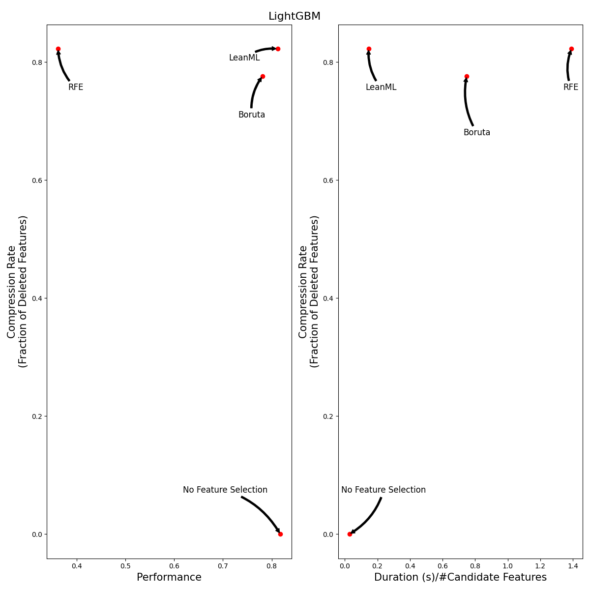
We compare feature selection methods from the perspective of model size, performance, and training duration. A good feature selection method should select as few features as possible, with little to no performance reduction, and without requiring too much compute resources.
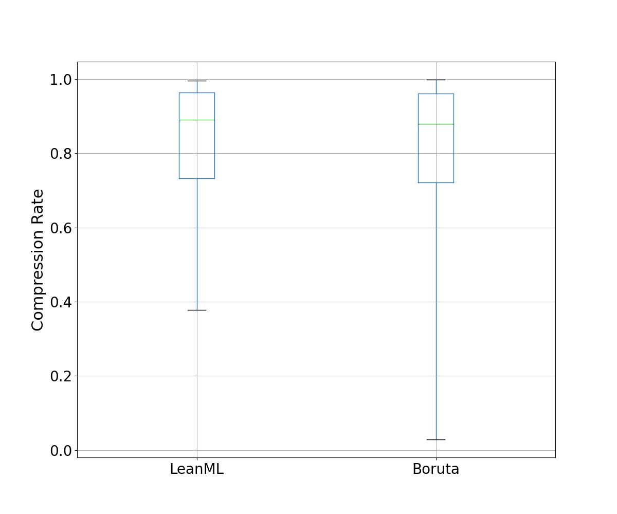
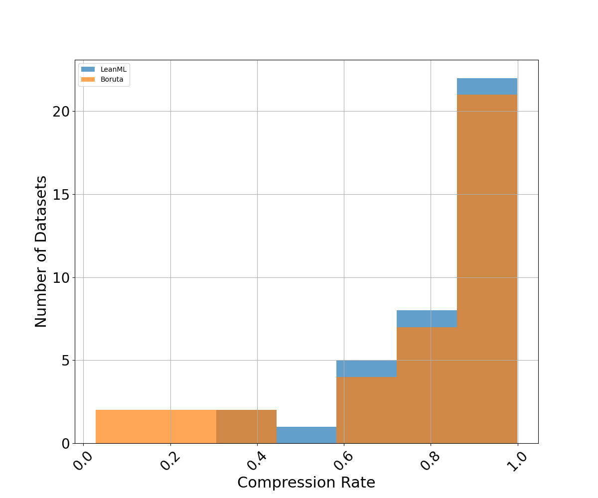
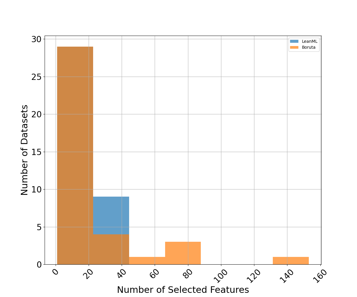
Model Size
We compare the number of features selected by each feature selection method. We also compare compression rates, defined as the fraction of candidate features a feature selection method did not select. For RFE, we use the same number of features as LeanML.
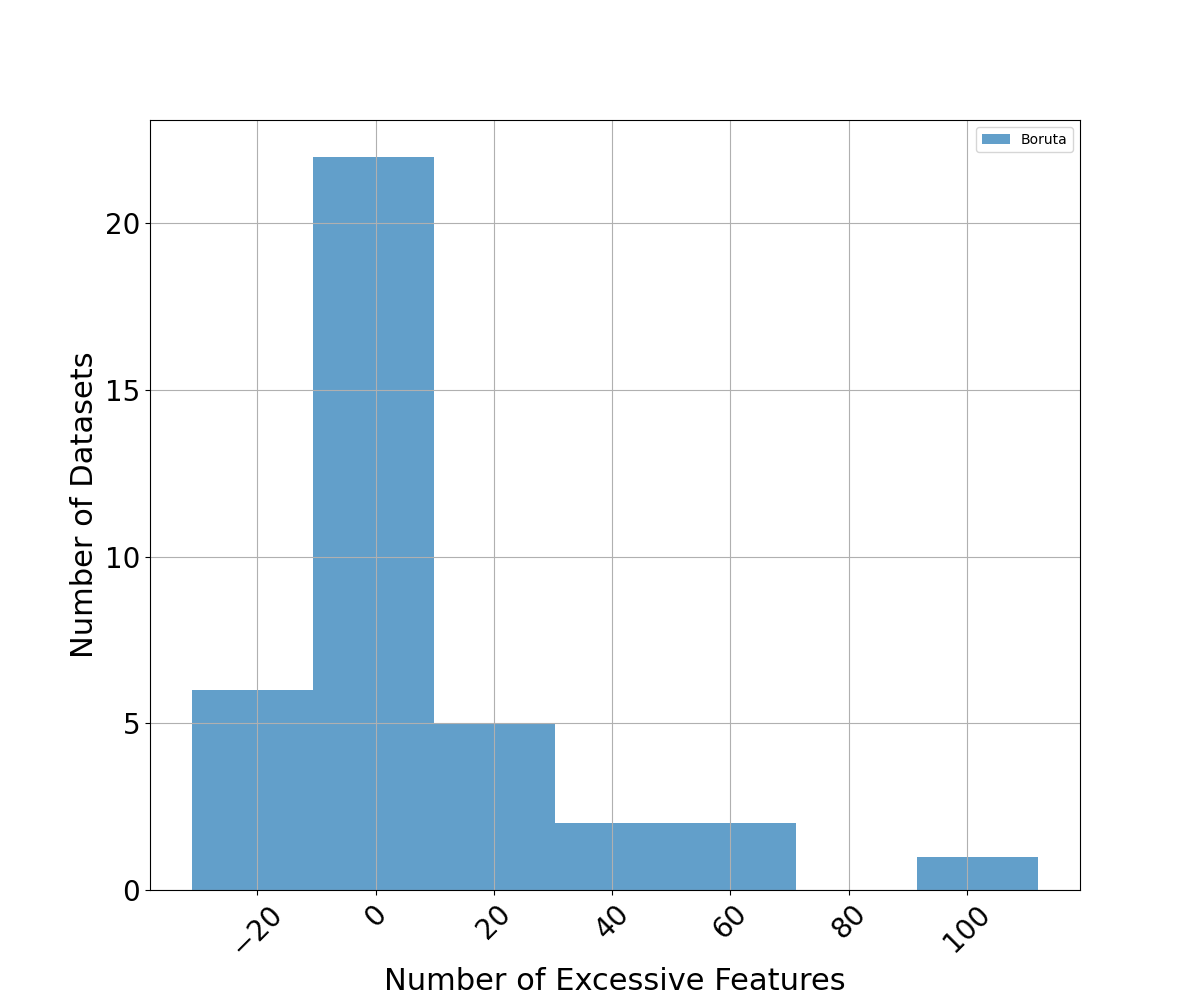
Results are illustrated in Figures 1, 2, 3, and 4 below.
LeanML is able to reduce the number of candidate features by 82% on average, compared to 78% for Boruta. Additionally, the number of features selected by LeanML rarely exceeds 20 and never exceeds 45.
Boruta on the other hand selected as many as 140 features. More importantly, it can be seen in Fig. 4 that Boruta almost always selected more features than LeanML, and selected up to 100 more features at times.
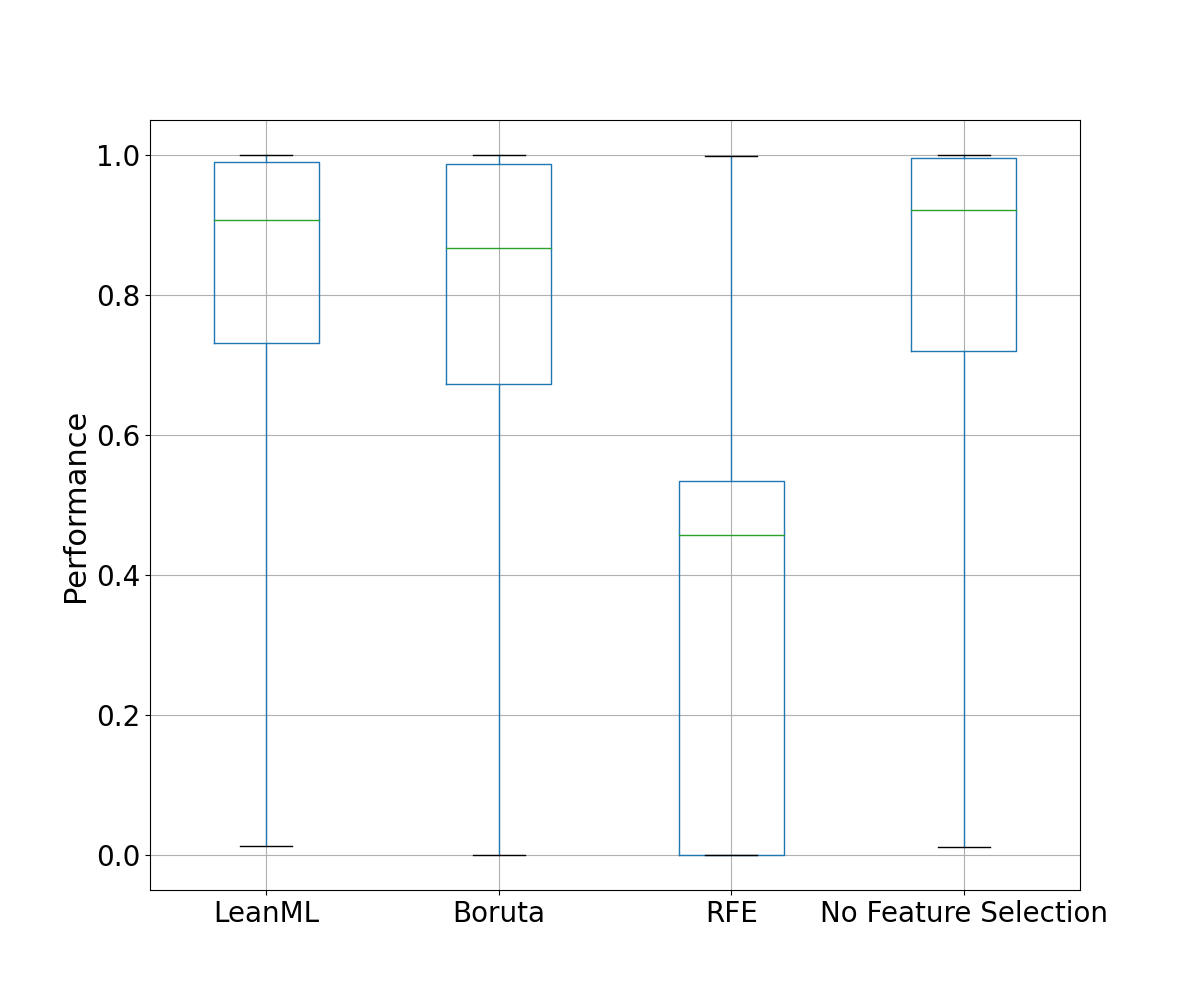
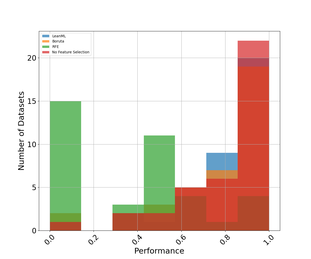
Performance
As the performance metric, we use the \(R^2\) for regression problems and the AUC for classification problems. These are evaluated on the testing set. See Figures 5 and 6 for results.
It can be seen that LeanML feature selection outperforms both Boruta and RFE out-of-sample, despite using far fewer features. We also see that LeanML is able to achieve the same performance as without feature selection on average with 82% fewer features, and often improves performance!
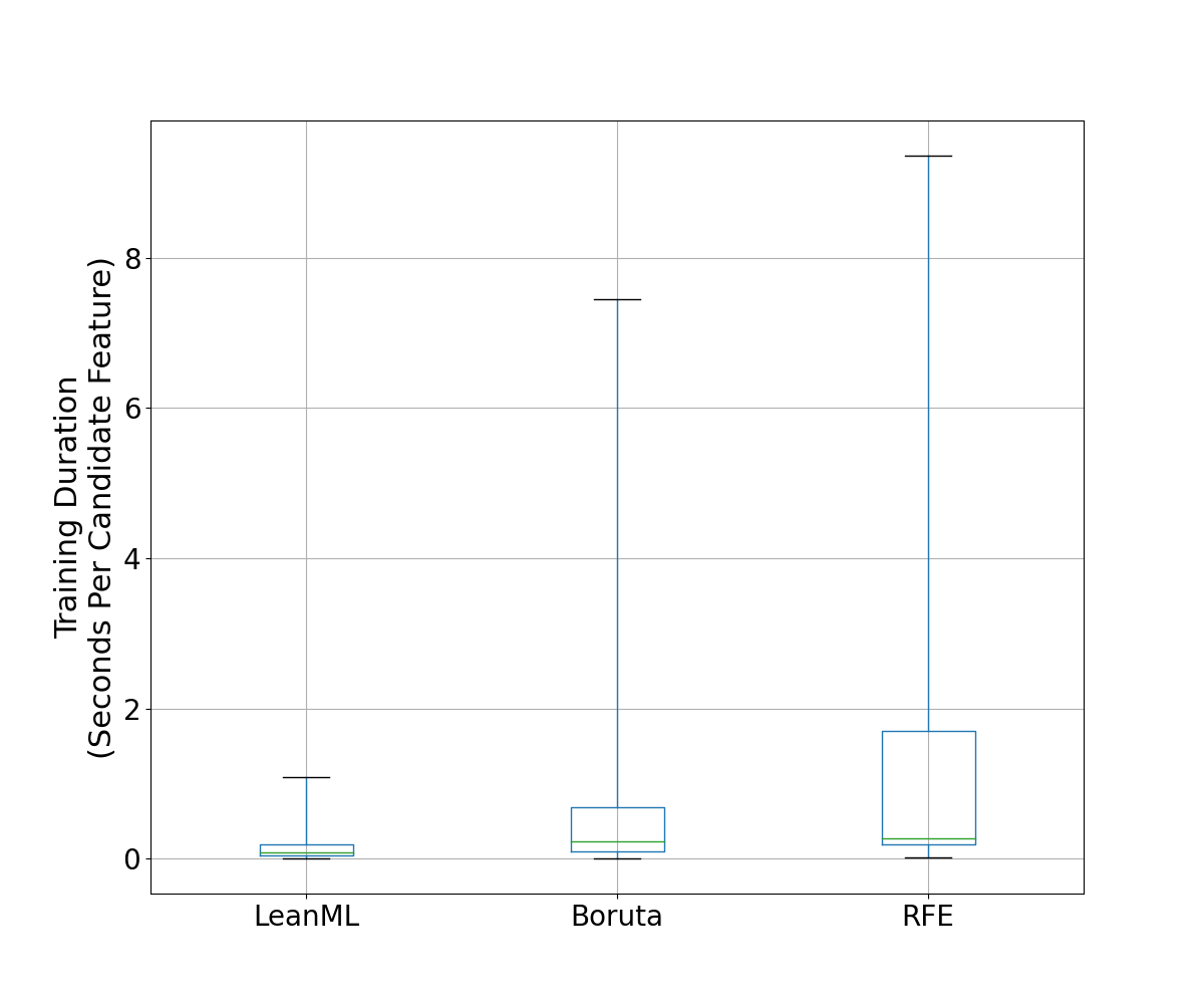
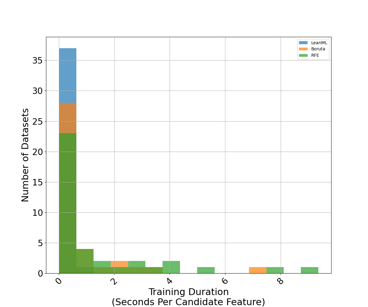
Training Duration
We compare the training duration (in seconds) of each method divided by the number of candidate features.
Results are illustrated in Figures 7 and 8 where it can be seen that, on average, training with LeanML feature selection took about 0.15 second per candidate feature, compared to 0.75 second for Boruta, and 1.39 seconds for RFE.
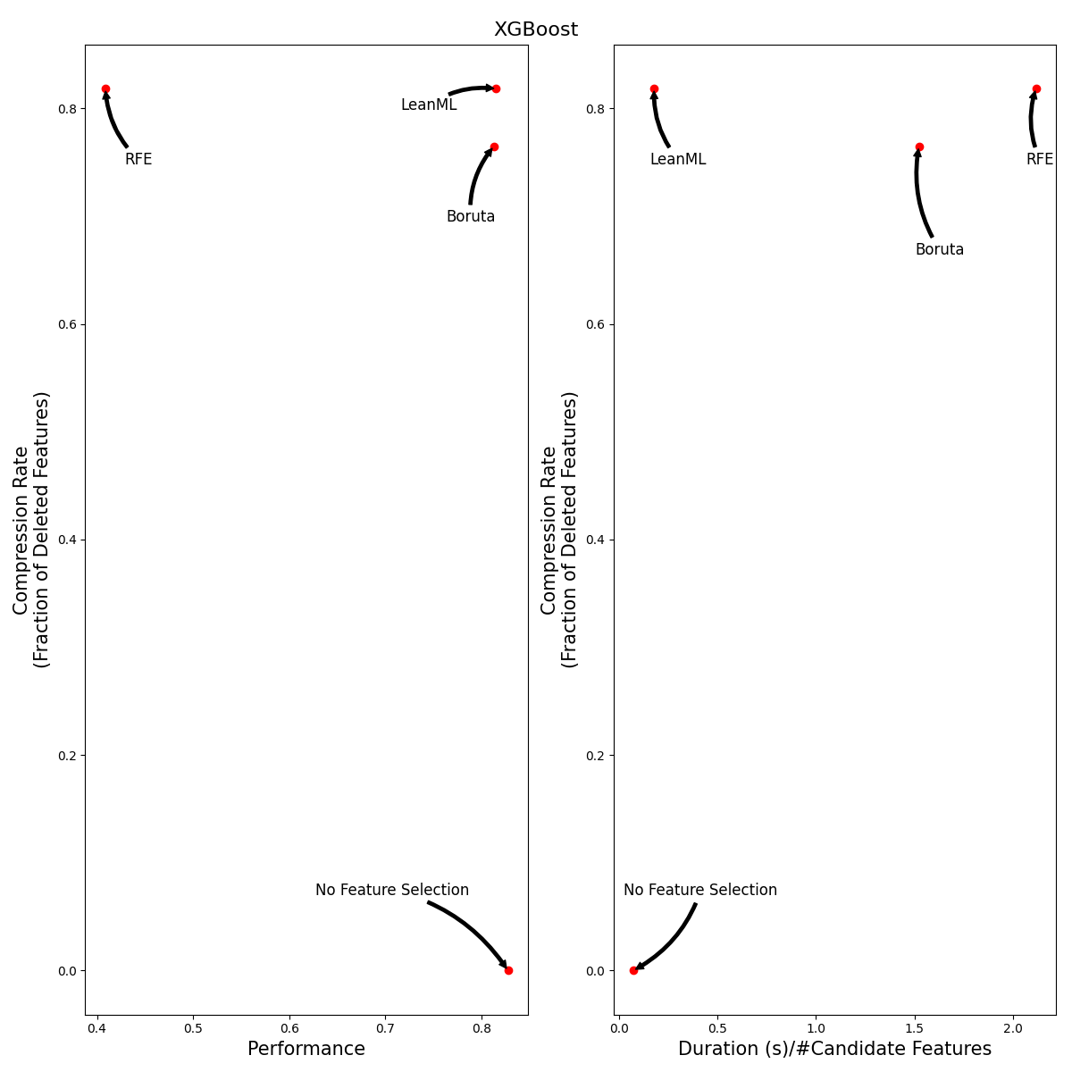
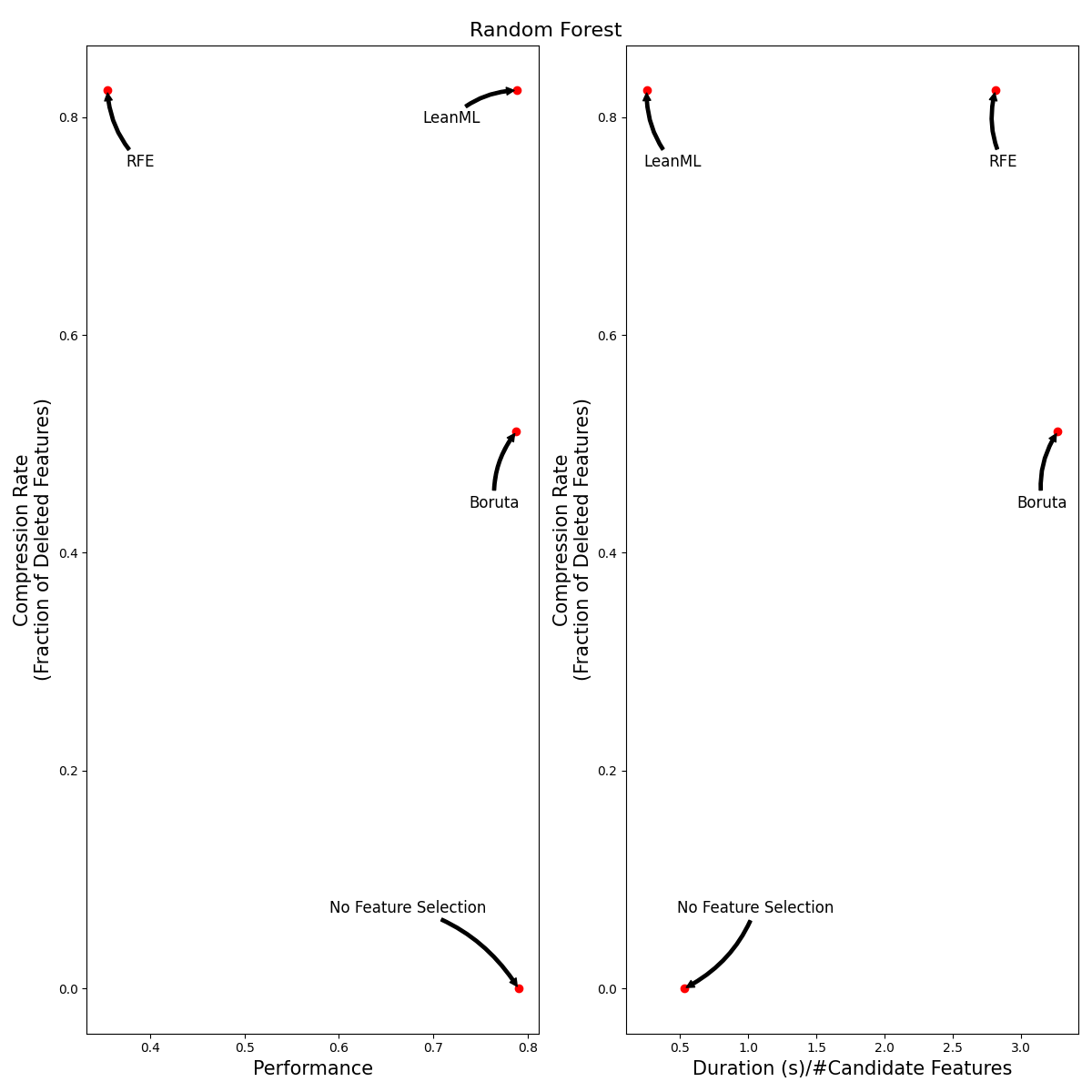
Beyond LightGBM
We ran the same experiments using XGBoost and Random Forest. Results are illustrated in the tables and figures below.
It can be seen that, out of the three feature selection methods, RFE is by far the worst! RFE is consistently the least accurate, and it is 100x slower than LeanML.
Boruta tends to be as accurate as LeanML on average, but it is 5 to 12 times slower and has a much lower compression rate, especially when wrapped around Random Forest. When wrapped around Random Forest, Boruta never selected fewer features than LeanML did. We found instance where Boruta selected up to 700 more features than LeanML.
As for LeanML, on average it consistently performs as well as without including feature selection, with 82% fewer features! When wrapped around Random Forest, LeanML is on average twice as fast.
| Model | No Feature Selection | LeanML | Boruta | RFE |
|---|---|---|---|---|
| LightGBM | 0.00 ± 0.00 | 0.82 ± 0.03 | 0.78 ± 0.04 | - |
| Random Forest | 0.00 ± 0.00 | 0.82 ± 0.03 | 0.51 ± 0.06 | - |
| XGBoost | 0.00 ± 0.00 | 0.82 ± 0.03 | 0.76 ± 0.04 | - |
| Model | No Feature Selection | LeanML | Boruta | RFE |
|---|---|---|---|---|
| LightGBM | 0.82 ± 0.04 | 0.81 ± 0.04 | 0.78 ± 0.04 | 0.36 ± 0.05 |
| Random Forest | 0.79 ± 0.04 | 0.79 ± 0.04 | 0.79 ± 0.04 | 0.35 ± 0.05 |
| XGBoost | 0.83 ± 0.04 | 0.82 ± 0.04 | 0.81 ± 0.04 | 0.41 ± 0.06 |
| Model | No Feature Selection | LeanML | Boruta | RFE |
|---|---|---|---|---|
| LightGBM | 0.03 ± 0.01 | 0.15 ± 0.03 | 0.75 ± 0.22 | 1.39 ± 0.35 |
| Random Forest | 0.53 ± 0.29 | 0.26 ± 0.06 | 3.27 ± 0.82 | 2.81 ± 0.63 |
| XGBoost | 0.07 ± 0.03 | 0.18 ± 0.05 | 1.52 ± 0.39 | 2.12 ± 0.51 |
| Model | No Feature Selection | LeanML | Boruta | RFE |
|---|---|---|---|---|
| LightGBM | 255 ± 72 | 0 ± 0 | 6 ± 4 | - |
| Random Forest | 255 ± 73 | 0 ± 0 | 53 ± 20 | - |
| XGBoost | 254 ± 72 | 0 ± 0 | 8 ± 5 | - |
Conclusion
We show how to seamlessly wrap LeanML, Boruta, and RFE feature selection around popular predictive models in Python, including but not limited to lightgbm, xgboost, tensorflow, and sklearn models.
Using 38 real-world classification and regression problems, we showed that LeanML feature selection cuts the number of features used by 82% on average, at no performance cost.
As an alternative, RFE can be up to 100 times slower on average than LeanML and performs significantly worse! RFE's notable poor performance is perhaps not surprising as RFE tends to exacerbate overfitting. Indeed, when a model is overfitted, it is often because of [...] the most important features! Thus, removing the least important features and keeping the most important ones can only amplify the problem.
As for Boruta, while it performs similarly to LeanML on average, it can be up to 12 times slower than LeanML on average, and almost always selects more features than LeanML, often hundreds.
Note: The source code to reproduce all experiments can be found here.